
📅 Originally Published: · Last Updated:
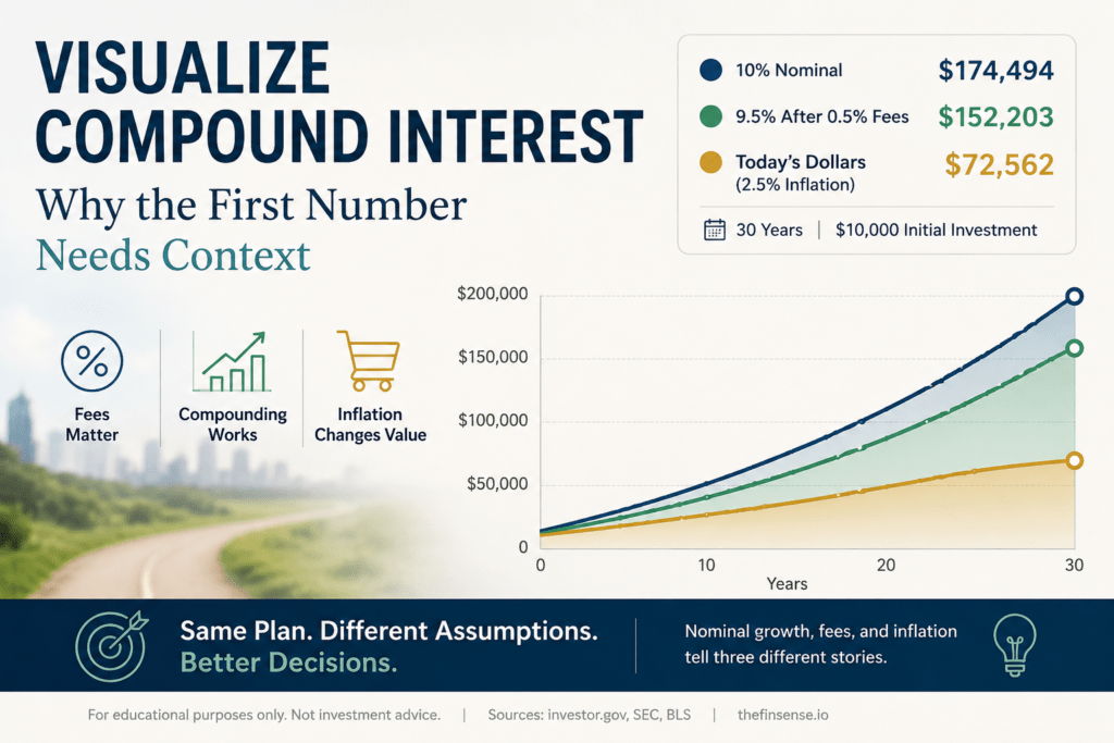
Answer first: For compound interest after fees and inflation, one future-balance number is not enough. Separate the nominal account balance, the balance after costs that are not already reflected in your return input, and the purchasing power of that money in today’s dollars. In this example, a $10,000 lump sum becomes $174,494 at a fixed 10% nominal return, about $152,203 after a 0.5% annual fee-drag assumption, and about $72,562 after a 2.5% inflation adjustment. Those figures describe the same modeled path in different ways; they should not be subtracted from one another as if every gap were an investment loss.
A compound interest calculator can do the math correctly and still leave you with the wrong planning number. Enter a starting balance, a return, and a time horizon, and you get future dollars. The mistake is treating that output as if it already reflected purchasing power and every cost you may pay.
Label the dollars before you use them. This guide follows one $10,000 lump-sum case across nominal dollars, fee-adjusted dollars, and dollars adjusted for inflation over three decades. The return, fee, and inflation inputs are fixed so the unit mismatch is easy to see; they are illustrations, not forecasts.
One Investment, Four Answers
Hold the starting balance and time horizon constant, then change only the way the result is measured. With the same $10,000 case in every row, the four outputs stop looking like conflicting forecasts and start reading as four different lenses.
| Planning Lens | Rate Used | 30-Year Result | What the Number Means |
|---|---|---|---|
| Nominal calculator output | 10.00% | $174,494 | Future account dollars before a separate fee or inflation adjustment |
| Fee-adjusted nominal path | 9.50% | $152,203 | Future dollars after treating 0.5% as an annual return drag |
| Fisher-adjusted purchasing power | 6.83% | $72,562 | Today’s-dollar planning value after the fee-drag and 2.5% inflation assumptions |
| Simple subtraction shortcut | 7.00% | $76,123 | Easy-to-audit approximation from 10.0% − 0.5% − 2.5% |
Want to test your own assumptions? Change the starting balance, horizon, nominal return, annual fee drag, or inflation rate below. The calculator keeps nominal future dollars, after-fee future dollars, and today’s purchasing power separate so the units do not get mixed.
Change the assumptions and keep future nominal dollars, after-fee dollars, and today’s purchasing power separate.
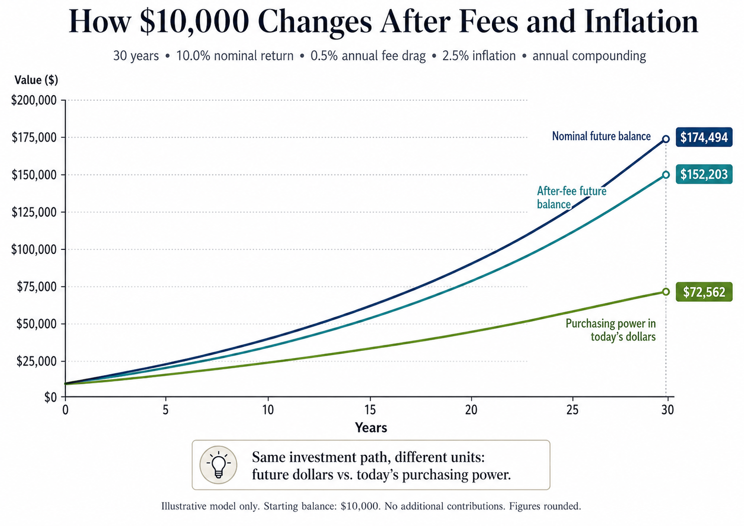
Each row answers a different question. The nominal result shows the future account balance under the stated return. The fee-adjusted result shows the modeled annual cost in future dollars. The Fisher row translates that path into today’s buying power, while the shortcut offers a planning estimate that is easier to calculate by hand.
That distinction changes the article’s main conclusion. Subtracting the Fisher-adjusted row from the nominal row does not produce a literal investment loss because the rows use different dollar units. What matters is what each number measures, not the raw gap between unlike units.
IN PLAIN ENGLISH:
Your future statement may show a six-figure balance while the same balance has much less buying power in today’s terms. Nothing disappeared from the account. The unit changed.
Why the Biggest Dollar Gap Is Not a Portfolio Loss
The SEC’s Investor.gov calculator asks for an initial investment, contributions, time, an estimated interest rate, a variance range, and compounding frequency. It is designed to show how money can grow. It does not include separate fields for inflation, advisory fees, fund expenses, taxes, or personal spending needs.
The calculator is doing its job: producing a nominal output from the inputs supplied. Trouble begins when that result is treated as if it were already a purchasing-power estimate. To use the result correctly, keep the units visible all the way through the math.
Compare Fee Drag in the Same Dollars
Under the article’s rate-drag convention, the modeled annual fee lowers the nominal return by half a percentage point. Both balances are future-dollar figures, so their $22,291 gap is a valid same-unit comparison.
Convert both paths with the same inflation assumption and the modeled fee difference becomes about $10,627 in today’s dollars. The fee did not create two separate losses. The table expresses the same modeled effect in two different unit systems.
| Fee Comparison | No-Fee Path | 0.5% Fee-Drag Path | Modeled Difference |
|---|---|---|---|
| Future dollars | $174,494 | $152,203 | −$22,291 |
| Today’s dollars at 2.5% inflation | $83,189 | $72,562 | −$10,627 |
The SEC warns that ongoing fees reduce the amount of money left in a portfolio to earn returns, and its investor bulletin shows that small annual fee differences can lead to large gaps in ending value. Isolate fee drag first, then convert the resulting balance for inflation.
The Tighter Formula and the 7% Shortcut
There are two useful ways to translate a nominal return into a real planning rate. The quick method subtracts the fee and inflation assumptions. The tighter method divides the after-fee growth factor by the inflation factor. The choice matters because the shortcut is easy to audit but comes out a little higher than the real result in this example.
Fisher planning rate: Start with the after-fee nominal rate, then divide its growth factor by the inflation factor. Under this article’s assumptions, ((1 + 10.0% − 0.5%) ÷ (1 + 2.5%)) − 1 = about 6.83%.
Quick calculation check: the Fisher case is $10,000 × (1.0682927)30 = $72,562, while the 7% shortcut gives $10,000 × (1.07)30 = $76,123.
The shortcut ends about $3,561, or 4.9%, higher because it subtracts inflation instead of dividing by the inflation factor. Use it as a quick screen; use the Fisher result when you want the tighter real-value estimate.
One More Precision Choice: How the Fee Is Applied
The base model treats the annual fee as a half-point reduction in return. A second method applies the fee to assets after the gross return, producing an effective nominal rate of about 9.45%. After the same inflation adjustment, the real rate is about 6.78% and the ending result is about $71,574. The difference is modest here, but it is another reason to label the calculation as a model.
Do Not Subtract a Fund Expense Twice
Your return input sets which fees still need to be deducted. A broad market index return generally does not reflect the expenses of the fund you use to track it. Fund expenses come out of fund assets, so they reduce the return investors receive. An advisor fee charged outside the fund may still need a separate adjustment. Check how the benchmark and fund returns are reported, along with your fee documents, before subtracting anything.
A common mistake runs in the opposite direction: starting with a return that already reflects the expense ratio, then subtracting the same cost again. When you visualize compound interest with a fund return, keep the index return, fund return, and personal account return as separate data layers. The S&P 500 ETF guide shows why that distinction matters.
Where Fees and Inflation Change the Decision
Fees and inflation alter the model in different places. Fees reduce the amount left to compound, while inflation changes what the ending dollars can buy. If you combine them into one haircut, you can no longer tell whether a lower result came from investment cost, lost buying power, or both.
Inflation Is an Assumption, Not a Current-Rate Label
The Bureau of Labor Statistics defines the Consumer Price Index as a measure of average price changes for a typical basket of consumer goods and services. BLS also notes that a national CPI average may not match one person’s experience. A household spending heavily on rent or medical care may face a different personal inflation rate.
The 2.5% input in this article is a long-term planning assumption. It is not presented as the latest CPI reading. Run at least one high-inflation case when the plan is sensitive to buying power, especially if much of your retirement spending falls in categories that often rise faster than the broad index. The inflation guide explains how different assets respond to that risk.
Use Total Annual Fee Load, Not One Convenient Line Item
The SEC separates costs into transaction fees and ongoing fees. Ongoing costs can include advisor fees, fund fees, plan fees, platform fees, and account fees. Your model should include only recurring costs that are not already reflected in the return series you chose.
For scale, moving from the nominal case to a 9% return path creates a $41,817 difference over the full horizon in the same future-dollar units. Treat that figure as the return hurdle an advisor service must justify, not as proof that every one-percentage-point fee is a bad deal.
| Scenario | Total Annual Fee Load | Inflation Assumption | Fisher-Adjusted Rate | $10,000 Ending Value |
|---|---|---|---|---|
| Low-cost case | 0.04% | 2.50% | 7.28% | $82,286 |
| Base case | 0.50% | 2.50% | 6.83% | $72,562 |
| Higher-cost stress case | 1.00% | 3.00% | 5.83% | $54,661 |
One headline number hides how sensitive the plan is to its inputs. Treat the rows as stress cases: if a small change in fees or inflation breaks the plan, the useful response is to revisit the savings target rather than defend the optimistic assumption. For a deeper look at advisor pricing, see the advisory-fee guide.
A Four-Step Workflow for Reading the Result
A spreadsheet is enough if the units, assumptions, and costs stay visible. Before a compound interest projection changes a savings or retirement decision, run it through these four checks.
- Choose the question before the rate. Decide whether you need a future account balance, a fee-adjusted balance, or today’s-dollar purchasing power. Write the unit next to the output so it cannot silently change later.
- Identify what the return already includes. An index return, fund return, and personal account return can reflect different costs. Subtract only fees that are not already embedded in the input.
- Apply fees and inflation in separate steps. Reduce the nominal return for the modeled annual fee load, then divide by the inflation factor for a tighter real-rate estimate. Keep the simple subtraction method as a quick cross-check.
- Run a range instead of trusting one forecast. Change the return, fee load, and inflation assumption one at a time. If the plan works only in the best case, the contribution target or timeline needs another look.
PRO TIP: Whenever you visualize compound interest, save three outputs beside the projection: nominal future dollars, fee-adjusted future dollars, and today’s dollars. That labeling habit prevents the unit mistake this article is built around.
Questions That Still Trip People Up
Should I subtract an ETF expense ratio from the return?
Only if the return input does not already reflect that fund expense. A broad index return usually does not include the ETF expense ratio, while a fund’s reported performance is reduced by its fund expenses. Start by checking whether your input is an index return, a fund return, or your own account return; then subtract only costs that sit outside that series.
What inflation rate should I use for a long-term projection?
Use an explicit planning assumption and test more than one case rather than treating today’s CPI reading as a permanent rate. The 2.5% figure in this article is only an example. Your spending mix can also differ from the national CPI basket, so a plan that is sensitive to purchasing power should also be tested with a high-inflation case.
What if returns, fees, or inflation change from year to year?
Then a fixed-rate compound interest model is a scenario, not a forecast. Its value is that it keeps the unit treatment transparent. For a more realistic plan, vary the inputs across scenarios or use a model with changing annual assumptions. Keep the same discipline: check what the return already includes, apply the remaining costs once, and keep the nominal and real dollar labels separate.
Bottom Line: Label the Dollars Before You Trust the Result
A standard calculator is useful for nominal growth. The planning error begins when that output is treated as today’s purchasing power or when a cost already embedded in the return is subtracted again.
Keep the sequence clean: calculate the nominal future balance, isolate fees in the same units, then convert the fee-adjusted path into today’s dollars. Use the 7% subtraction shortcut for speed and the Fisher adjustment for a tighter estimate. Do not describe the subtraction between nominal future dollars and today’s dollars as a literal portfolio loss.
Before the result changes how much you save, write the unit beside it and rerun the model with less favorable assumptions. If the plan survives only the best case, the weakness is in the plan, not in the calculator.
YOUR TURN
When you look at your own projection, is the ending number labeled as future dollars or today’s purchasing power?
Update history
- v1.6 2026-08-23 REMEDIATION
Refocused the article on reading compound-interest results after fees and inflation, removed tangential brokerage and Rule of 72 material, reduced repetitive FAQ coverage, and migrated the trust package to the current canonical markup.
- v1.5 2026-07-28 SEO
Removed an outdated search-title promise, converted editorial links to canonical URLs, and clarified how fund expenses affect reported returns.
- v1.4 2026-07-26 METHOD
Split the methodology into a concise result-adjacent summary and a full reproducible method in the bottom evidence package.
- v1.3 2026-07-11 CORRECTION
Corrected the nominal-versus-real unit mismatch, promoted the Fisher adjustment, clarified fee double counting, and refreshed the evidence package.
- v1.2 2026-07-10 TRUST
Added article-specific author, evidence, method, disclosure, and internal-link surfaces.
- v1.1 2026-07-09 DATA
Updated the nominal, fee-drag, and sensitivity figures and removed redundant large-number callouts.
- v1.0 2026-03-16 PUBLISH
Original publication of the compound-interest visualization guide.