
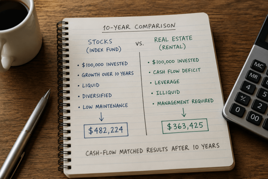
📅 Originally Published: · Last Updated:
Answer first: Under the base assumptions, the S&P 500 wins the timing-adjusted comparison. The rental earns an estimated 6.41% internal rate of return (IRR), below the model’s 10.37% index return. Gross equity points the other way because it ignores the owner’s annual cash shortfalls and sale friction. These are scenario outputs, not forecasts; a better purchase price, stronger rent economics, cheaper financing, or faster appreciation can reverse the result.
The stocks vs real estate argument often starts with identity: are you a stock person or a property person? That framing hides the useful question. If the same household has $100,000 available today, which path creates more wealth after financing, operating costs, additional cash contributions, liquidity limits, and selling friction are put on the same timeline? Taxes are discussed separately because the result depends heavily on the owner, account, and jurisdiction.
The homeowner wealth gap is real but easy to misuse. The Federal Reserve’s 2022 Survey of Consumer Finances reported median net worth of $396,200 for homeowners and $10,400 for renters and other non-homeowners. That is a snapshot across households, shaped by age, income, credit access, saving habits, and years of ownership. It does not prove that the next rental available to you will beat a low-cost index fund.
This article treats the rental as a business. It gives the property credit for leverage, rent, and mortgage paydown, while charging it for property costs, debt service, extra cash required, and an assumed sale cost. The stock path includes the fund fee and uses the same cash-flow timing. Purchase costs and owner-specific taxes stay outside the headline comparison.
The $100K Head-to-Head After Operating, Financing, and Sale Costs
Both investors begin with identical capital. Investor A buys a $100,000 position in the Vanguard S&P 500 ETF (VOO) and reinvests distributions. The model uses a 10.40% gross annual return and subtracts VOO’s 0.03% annual fund fee, producing a 10.37% net assumption. S&P Dow Jones Indices has described the index’s long-run total return as roughly 10% since its 1957 launch, while its December 2024 market commentary cited 10.5% for the longer series beginning in 1926. The 10.40% input is a historical-style scenario, not a forecast.
Investor B uses the $100,000 as a 20% down payment on a $500,000 single-family rental and finances $400,000 at 6.30% fixed for 30 years. Freddie Mac recorded 6.30% on April 16 and April 30, 2026; its national Primary Mortgage Market Survey (PMMS) average was 6.65% on August 20, 2026. PMMS uses a narrow borrower profile: conventional conforming purchase loans on owner-occupied, one-unit homes, with 75% to 80% LTV and FICO scores of 740 or above. The model uses 6.30% only as a dated benchmark, not as a rental-property quote. A real deal should use the lender’s investment-property rate, points, fees, and terms.
Base-Case Operating Assumptions
| Rental Input | Annual Amount | How It Enters the Model |
|---|---|---|
| Gross rent | $36,000 | $3,000 per month, held flat for the base case |
| Property tax | $5,500 | Operating expense |
| Insurance | $2,500 | Operating expense |
| Maintenance and CapEx reserve | $5,000 | Operating expense and reserve assumption |
| Vacancy allowance | $2,880 | 8% of gross rent |
| Property management | $3,600 | 10% of gross rent |
| Net operating income | $16,520 | Gross rent minus operating expenses |
| Mortgage principal and interest | $29,711 | $2,475.89 per month |
| Annual cash flow after debt service | −$13,191 | Additional owner cash required each year |
The property starts with a 3.30% cap rate: $16,520 of net operating income on a $500,000 purchase price. Annual mortgage payments equal 7.43% of the original loan balance, and the debt-service coverage ratio is only 0.56. The rent economics cover barely more than half of scheduled debt service, so leverage starts out negative in this case.
Four Views of the Same 10-Year Outcome
| Year 10 View | Rental Property | S&P 500 Path | What the Comparison Shows |
|---|---|---|---|
| Gross equity | $424,365 | $268,232 | Rental appears ahead by $156,133 |
| Net sale equity after assumed 8% exit cost | $363,425 | $268,232 | Rental appears ahead by $95,193 |
| Simple net-of-cash-added view | $231,518 | $268,232 | Index ahead by $36,714 |
| Cash-flow-matched terminal wealth | $363,425 | $482,224 | Index ahead by $118,799 |
| Timing-adjusted annual return | 6.41% IRR | 10.37% model input | Rental return falls below the modeled index hurdle |
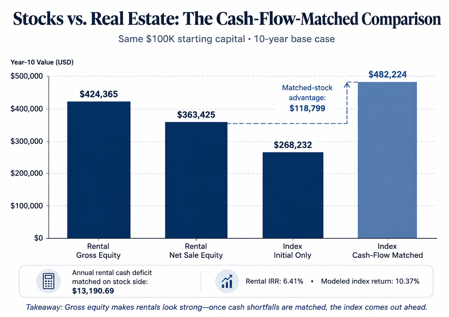
Both paths use the same starting capital over a 10-year horizon. The rental model assumes leveraged property exposure financed with a 30-year fixed mortgage, flat rent and operating costs, a historical-style appreciation rate, and an exit-cost allowance. The stock path uses the article’s net index-return assumption and receives the same year-end cash contributions as the rental’s annual deficits. Purchase costs and income taxes are excluded. These are scenario outputs, not forecasts.
WHAT CHANGES THE RESULT?
The rental can beat the modeled index hurdle, but only when financing, appreciation, rent economics, or purchase price improve enough. The table changes only the mortgage rate and appreciation rate; all other assumptions remain fixed.
| Mortgage / Appreciation | Annual Cash Deficit | Net Sale Equity | Rental IRR | Result vs 10.37% Index Assumption |
|---|---|---|---|---|
| 5.0% / 4.3% | −$9,247 | $375,443 | 8.94% | Index hurdle remains higher |
| 6.30% / 4.3% | −$13,191 | $363,425 | 6.41% | Base case favors index |
| 6.30% / 5.5% | −$13,191 | $448,361 | 9.35% | Closer, but still below index hurdle |
| 5.0% / 5.5% | −$9,247 | $460,378 | 11.64% | Rental clears the modeled hurdle |
Use the calculator below with a real listing and lender quote. It applies the same cash-flow-matching rule as Table 2: when the rental requires extra cash, the index receives the same year-end contribution; when the rental distributes cash, the index side makes the same withdrawal.
Rental vs. Index Fund Calculator
Compare one leveraged rental with an index fund using the same starting capital and the same year-end household cash-flow schedule.
Matched index $482,224 vs. net rental sale equity $363,425.
| Metric | Result | What it means |
|---|---|---|
| Net operating income | $16,520 | Before financing |
| Cap rate | 3.30% | NOI ÷ property price |
| First-year DSCR | 0.56x | NOI ÷ scheduled debt service |
| First-year rental cash flow | −$13,191 | After debt service |
| Exit property value | $761,751 | At the entered appreciation rate |
| Exit mortgage balance | $337,386 | After the entered holding period |
| Rental IRR | 6.41% | Timing-adjusted rental return |
| Break-even appreciation | 5.95%/yr | Property growth needed to match the index ending value |
Cash-flow matching: the index starts with the same down payment. Each year it receives the same amount the rental requires from the owner, or makes the same withdrawal when the rental distributes cash.
Scope: rent and operating-cost inputs are held flat; purchase closing costs, income taxes, HOA fees, unusual repairs, refinancing, and personal-use value are excluded. Scenario tool only; not a forecast or lender quote.
Under the same year-end cash-flow schedule, the stock-side break-even return is about 6.41% net per year. A lower realized stock return would narrow or reverse the base-case advantage, while a higher return would widen it.
Table 2 changes once the owner’s added cash gets an opportunity cost. Gross equity is only a balance-sheet snapshot; it does not show how much extra cash the owner put in or what that money could have earned elsewhere. Once timing is counted, the base-case rental looks less like a runaway winner and more like a leveraged deal earning a mid-single-digit return.
Why Gross Equity Gives the Wrong Answer
The usual comparison puts home-price growth on one side and stock total return on the other. Those are different measures. The Federal Housing Finance Agency (FHFA) Purchase-Only House Price Index tracks repeat-sale price changes for single-family homes. It does not subtract property tax, insurance, maintenance, vacancy, management, financing, or selling expenses. A fund’s published return, by contrast, already reflects the expense ratio charged inside the fund.
The FHFA/FRED index was 441.30 in April 2026, with January 1991 set to 100. From that starting point, the long-run nominal price growth is about 4.3% per year. That is useful as a historical model input, but it is not a rental return. A rental also depends on income, leverage, later cash added, purchase price, and exit costs.
The same point applies to leverage. A 20% down payment creates five times the property exposure, so the base price-growth assumption adds $21,500 of gross value in Year 1. The owner also carries the full cost stack and a $400,000 loan. Leverage magnifies the asset; it does not erase a weak deal.
IN PLAIN ENGLISH
Do not compare a home’s headline appreciation rate with a stock index’s total return. First turn the property into a stream of dated cash flows: down payment, rent, operating expenses, debt service, repairs, taxes, and sale proceeds. Then calculate IRR or compare those cash flows with what the same money could have earned in the alternative investment.
The Exit-Cost Assumption Is Material
This model applies an 8% sale-cost assumption to the Year 10 property value. It is not a fixed fee schedule: agent pay is negotiable, and taxes, concessions, repairs, staging, and local closing charges vary. The model needs an exit allowance because property sales have meaningful friction, while a liquid ETF can often be sold without a brokerage commission. In the base case, the assumed sale cost removes $60,940 from equity.
Taxes Can Help During the Hold and Hurt at Exit
Under federal tax rules, residential rental buildings generally use a 27.5-year depreciation period, while land is not depreciable. Depreciation can lower taxable rental income during the hold, but a sale can also create unrecaptured Section 1250 gain, subject to a maximum 25% federal rate. The final tax bill depends on basis, passive-loss limits, income, state law, and deal structure, so the headline comparison does not force one after-tax result onto every owner.
When Real Estate Leverage Starts Working
Leverage helps when the property can carry the debt and still earn a return on the owner’s equity. The base-case rental does not meet that test. Its 3.30% cap rate sits far below its 7.43% mortgage constant, and its 0.56 debt-service coverage ratio means the owner must add cash every year.
Even so, leverage creates a real early benefit. In Year 1, the property gains $21,500 under the base price-growth assumption, while mortgage paydown adds about $4,643 of equity. After the annual cash deficit, the rough first-year gain is about $12,952 before purchase costs, taxes, and sale friction. The modeled index gain is $10,370. Real estate can lead early even with negative cash flow.
The danger is treating early paper equity as proof of a better long-term investment. A property with weak rent economics becomes dependent on price growth. That can work, as the sensitivity table shows, but the thesis has shifted from rental income to a leveraged bet on local prices.
What the Base-Case Metrics Are Warning You About
- 3.30% cap rate: the property produces $16,520 of NOI on a $500,000 price. That sits well below the loan’s cost, so price growth is doing more of the work.
- 0.56 debt-service coverage ratio: operations do not cover the mortgage; the owner has to keep supplying cash.
- 6.41% levered IRR: once the down payment, yearly deficits, and net sale proceeds sit on one timeline, the base case finishes below the modeled 10.37% stock hurdle.
Cash-on-cash return tells the same first-year stress story from another angle: it is about −13.2% before tax because the owner must add that share of the original down payment each year. It is a useful warning light, but the full cash-flow timeline still decides the case.
The Advantage of Low-Friction Stock Compounding
A low-cost index fund has no tenant, property-tax bill, vacancy period, contractor call, refinance decision, or single-address risk. Cash payouts can be reinvested, and fractional shares let nearly every dollar stay invested. That lower friction matters here because the stock path can keep compounding while the rental keeps asking the owner for cash.
VOO’s 0.03% annual fund fee reduces the model’s 10.40% gross assumption to 10.37%. On the starting lump sum over ten years, the difference between those two rates is about $730. That small direct fee does not guarantee a high return, but it leaves more of the market’s result in the investor’s account. The larger risk is behavior: selling during a crash can ruin the advantage of a sound long-term plan.
The same low friction makes the matched-cash comparison useful. If the rental owner must supply the shortfall at each year-end, the stock investor can put in the same cash. Under the model, those deposits grow the index balance to about $482,224. The rental ends with $363,425 after the assumed sale cost. The gap comes from giving both paths the same cash schedule, not from assuming the stock investor saves more.
For readers who want to inspect the compounding math, visualizing compound interest after fees and inflation shows how timing and repeat deposits change the ending value. That matters in a stocks vs real estate comparison because property cash calls rarely arrive as one neat lump sum.
PRO TIP: Underwrite a real purchase with the lender quote for a non-owner-occupied property. PMMS can frame a scenario, but its tightly filtered owner-occupied loan profile should not be treated as the rate available on a rental.
The Four-Part Stocks vs Real Estate Decision Filter
1. Protect the liquidity horizon first.
Money that may be needed for an emergency, tuition, a home purchase, a move, or another near-term goal should not go into a direct property just because the forecast looks good. Property sales take time and carry uncertain costs. A broad ETF can also fall sharply, but it can usually be sold in pieces instead of all at once.
2. Underwrite the property before forecasting price growth.
Use the actual purchase price, a lender quote, local taxes, an insurance quote, market rent, a vacancy allowance, repair reserves, management costs, HOA charges, and purchase closing costs. Calculate cap rate, debt-service coverage, and first-year cash-on-cash return before adding a price-growth assumption. A deal that fails without strong price growth is a price bet, not an income thesis.
3. Compare returns on the same timeline.
Build annual or monthly cash flows for the down payment, purchase costs, net rent, debt service, major repairs, taxes, and net sale proceeds. Calculate the rental IRR. Then compare it with a sensible hurdle for the other portfolio instead of assuming stocks must deliver their historical average. Also run a matched-cash stock path so every extra dollar sent to the property gets an opportunity cost.
4. Charge for concentration and work.
One rental ties capital to one building, neighborhood, tenant market, insurer, and local economy. It also brings hands-on work and legal duties. Those costs do not need a fake precision number, but they should raise the return hurdle. A property can still be the better choice when the buyer has a sourcing edge, renovation skill, local knowledge, better financing, or a personal reason to own it.
| What You Find | Likely Interpretation | Next Step |
|---|---|---|
| Capital may be needed within five years | Direct-property liquidity risk is high | Keep this capital in an appropriately liquid allocation |
| DSCR below 1.0 and thin reserves | The property depends on owner cash infusions | Reprice the deal, improve financing, or walk away |
| Rental IRR below the portfolio hurdle | Leverage and appreciation do not compensate for the cash-flow burden | Prefer the simpler portfolio unless nonfinancial benefits matter |
| Rental IRR clears the hurdle with conservative inputs | The specific deal may justify its illiquidity and work | Stress-test repairs, vacancy, taxes, and exit value before committing |
| Property provides diversification but not a return edge | It may still serve a portfolio role | Size it around concentration, reserves, and personal capacity |
Cash waiting for a purchase also deserves a separate plan. Protecting short-term savings from inflation is not the same decision as choosing between long-duration stocks and a leveraged rental.
FAQ: Stocks vs Real Estate
Is real estate or the stock market better for long-term wealth?
Neither wins in every case. A diversified index fund is liquid, cheap, and easy to scale, while direct property can add leverage, rental income, tax benefits, and a local sourcing or renovation edge. The useful comparison is the return on the property’s dated cash flows versus a reasonable hurdle for the other portfolio. In this article’s base case, the index wins after the rental’s annual cash shortfalls and sale friction are matched on the same timeline; stronger property economics can reverse that result.
Does mortgage principal paydown count as a return?
Principal paydown increases owner equity, so it belongs in the economic result. It is not free money, however. The principal comes from mortgage payments funded by the property’s net operating income and, when cash flow is negative, by additional owner contributions. A proper model includes the full debt payment in annual cash flow and captures the lower mortgage balance in the sale proceeds or terminal equity.
Should I use historical average returns in my decision?
Use historical returns to build scenarios, not as promises. The 10.40% stock return and 4.3% property-appreciation rate here are historical-style assumptions. A real decision should test lower stock returns, weaker appreciation, changing rents and expenses, vacancy, repairs, and different sale dates. The property should not require one optimistic input to work, and the stock investor should not rely on the historical average arriving smoothly.
The Bottom Line: Compare Cash Flows, Not Asset-Class Stories
The base case looks like a real-estate win if you stop at $424,365 of gross equity. Complete the ledger, however, and the picture changes: assumed sale friction reduces the rental to $363,425, while giving the stock strategy the same annual cash contributions lifts its terminal value to about $482,224. The rental’s timing-adjusted return is about 6.4% before purchase costs and taxes.
That is not a verdict against real estate. The sensitivity table shows the rental clearing the modeled stock hurdle when financing and appreciation improve enough, and a better purchase price or stronger rent economics can do the same. The point is narrower: give leverage credit only after every cash call and exit cost is counted.
Before buying, model the property’s dated cash flows, calculate IRR, and give the alternative portfolio the same contributions. If the deal still clears the higher return hurdle you require for poor liquidity, single-property risk, and hands-on work, it may earn a place. If it works only under aggressive appreciation, reprice the deal or walk away.
YOUR TURN
Take one property you have seriously considered and list every dated cash flow, including purchase costs and annual shortfalls. Does its IRR still clear the return hurdle you would require from a concentrated, illiquid investment?
Update history
- v1.7 2026-08-23 ENHANCEMENT
Embedded the rental-vs-index calculator directly in the article body with an isolated, fail-visible runtime so it cannot be claimed by the shared calculator engine. Core base-case assumptions and published comparison outputs were unchanged.
- v1.6 2026-08-23 MAINTENANCE
Corrected the revised April FHFA/FRED HPI value to 441.30, refreshed PMMS context through August 20, 2026, trimmed glossary-like and repetitive sections, and migrated the bottom trust package to the current canonical DOM.
- v1.5 2026-07-27 FACT CHECK
Corrected the PMMS eligibility description to the official loan-to-value and FICO filters, normalized internal links, narrowed an unsupported FAQ statement, and reduced repetitive cash-flow guidance.
- v1.4 2026-07-26 MAINTENANCE
Clarified that PMMS is an owner-occupied benchmark rather than an investment-property quote, added the stock-side break-even rate, and refreshed mortgage-rate context.
- v1.3 2026-07-11 METHOD
Added cash-flow matching and rental IRR, removed stale outputs and unsupported thresholds, and rebuilt the decision framework around property-level metrics.
- v1.2 2026-07-10 MAINTENANCE
Standardized internal links, removed the embedded video, reduced duplicate boxes, and rebuilt the bottom trust package.
- v1.1 2026-07-09 FACT CHECK
Rechecked primary-source inputs and rebuilt the mortgage and investment calculations.
- v1.0 2026-03-16 PUBLISH
Original publication of the stocks vs real estate comparison.