
Updated:
📅 Originally Published:
The Bottom Line, Up Front
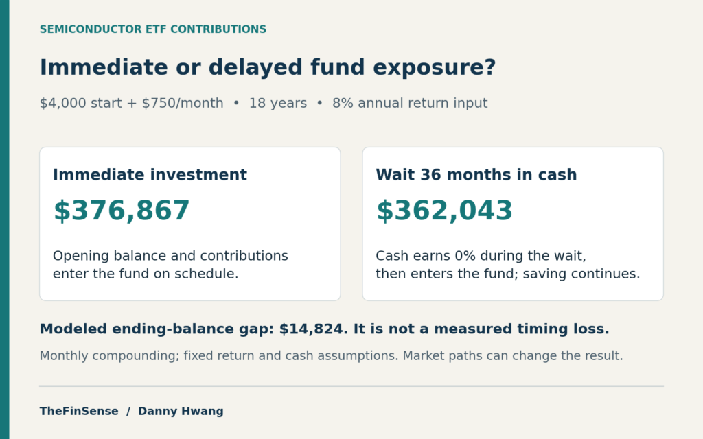
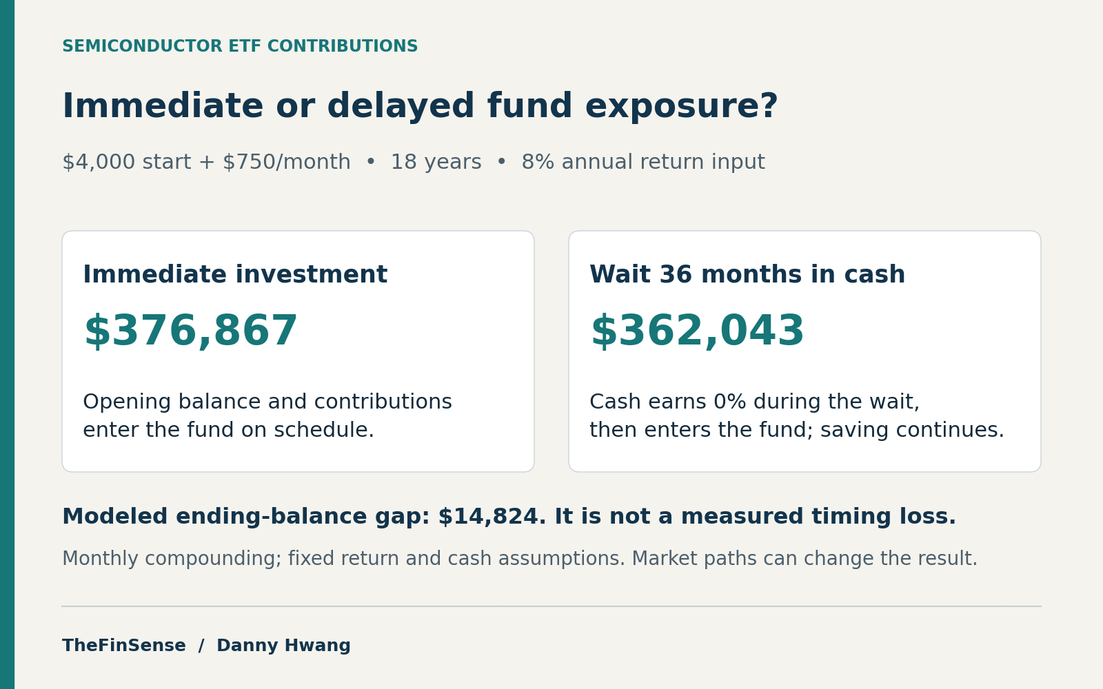
Semiconductor ETF dollar cost averaging means investing a fixed amount on a schedule. In the 18-year constant-return scenario below, a three-year wait produces a $14,824 lower ending balance with idle cash, or a $7,729 gap when waiting cash earns 4%. These are assumption-driven comparisons, not measured timing losses. A falling market or a higher cash return can change the result.
What is semiconductor ETF dollar cost averaging?
Semiconductor ETF dollar cost averaging means buying a fixed dollar amount of a chip fund like SOXX or SMH on a schedule regardless of price. The sector has a history of booms and downturns, but their timing is not a fixed clock.
Fabrication projects require substantial capital and construction time, so capacity decisions can meet a different demand environment when production begins. A monthly schedule removes discretionary entry-date decisions but leaves the investment exposed to sector losses. Staging an available lump sum can lag immediate investment when prices rise; investing new income as it arrives is a separate decision.
Browse the full guide
Choose the decision first: invest new income on a schedule, stage an available lump sum, or delay exposure in cash. Check reserves, horizon and sector concentration before comparing returns. The research context follows the practical route. Methodology.
This guide separates a recurring-investment plan from the decision to delay money already available. First check whether a concentrated sector sleeve fits your portfolio, then use the model to test the assumptions behind waiting.
A sharp chip selloff can prompt a choice between scheduled purchases and waiting. TheFinSense’s 36-month delayed-start calculation shows one outcome under stated return and cash-rate assumptions; it does not establish the cost of waiting through every market path.
How do you dollar cost average into a semiconductor ETF?
A working plan never asks you to name the bottom. That is the entire design goal, and it is why the mechanics below are boring on purpose.
How do you start dollar cost averaging into a semiconductor ETF?
For new monthly income, set an amount and date only after deciding that the semiconductor sleeve fits your allocation and risk capacity. Micah’s $750 purchase is a hypothetical plan, not a universal starting amount. A broad sector ETF still concentrates the portfolio in one industry.
Record the purchase schedule and the conditions for changing it in a written investment policy statement.
The calculator compares immediate investment with delayed fund exposure while saving the same amounts. During the wait, the opening balance and each monthly contribution stay in cash at 0%; at the end of the wait, the accumulated cash enters the fund at once and monthly investing continues. It accepts nonnegative fund-return assumptions; the separate table also tests 4% cash.
Compare immediate and delayed fund exposure. The widget holds waiting cash at 0% and accepts nonnegative fund returns; the table separately shows 4% cash. Defaults use the 18-year illustrative plan explained in the case below.
| Year | Steady | Wait | Gap |
|---|---|---|---|
| Year 5 | $61,067 | $55,809 | $5,258 |
| Year 10 | $146,088 | $138,255 | $7,833 |
| Year 15 | $272,756 | $261,086 | $11,670 |
| Year 18 | $376,867 | $362,043 | $14,824 |
At the displayed defaults, a longer delay increases the gap because the assumed fund return exceeds the fixed 0% cash rate. This widget does not test negative fund returns or a different cash yield. Outside the widget, if the fund return is 0% and waiting cash earns 0%, both schedules end at $166,000: $4,000 + 216 × $750. If the fund instead earns a constant −2% nominal annual rate (divided monthly) while cash earns 0% during the 36-month wait, delayed exposure finishes ahead; the formula in the method applies to that separate hypothetical case.
How much does waiting for the bottom actually cost?
Waiting 12 months for a clearer entry costs Micah about $2,597 on this 18-year plan. Waiting 60 months more than doubles the gap to roughly $34,023. Under this constant positive-return scenario, the delayed path never catches up. A different market path or cash return can shrink or reverse the gap.
What if you can’t stomach buying during a drawdown?
If the sector fits the plan but one entry date feels unmanageable, a written schedule can spread purchases. Each purchase still carries sector risk, and a schedule does not guarantee a better result.
When should you pause dollar cost averaging?
Pause or reduce scheduled purchases when the money is needed sooner, reserves are inadequate, or a sector position exceeds its written risk limit. A market view alone is a different reason and needs its own tested rule. The billings paper cannot tell you how often pausing ETF purchases succeeds. Buying during a decline can still incur losses, and averaging does not remove concentration risk.
Sensitivity table: 12 scenarios
Each row changes one assumption and holds the rest; read down to find the case closest to your own plan and horizon.
| Scenario | What changed | Steady schedule | Delayed start | Gap |
|---|---|---|---|---|
| Base case | balance $4,000, monthly $750, horizon 18y, return 8%, wait 36mo | $376,867 | $362,043 | $14,824 |
| Shorter wait | wait 12mo | $376,867 | $374,270 | $2,597 |
| Two-year wait | wait 24mo | $376,867 | $369,198 | $7,669 |
| Four-year wait | wait 48mo | $376,867 | $353,156 | $23,711 |
| Five-year wait | wait 60mo | $376,867 | $342,844 | $34,023 |
| Lower return | return 5% | $271,722 | $265,992 | $5,730 |
| Higher return | return 11% | $534,160 | $501,225 | $32,935 |
| Smaller monthly | monthly $400 | $208,837 | $199,263 | $9,574 |
| Larger monthly | monthly $1,000 | $496,888 | $478,315 | $18,573 |
| Shorter horizon | horizon 10y | $146,088 | $138,255 | $7,833 |
| Longer horizon | horizon 25y | $742,630 | $716,727 | $25,903 |
| Cash earns 4% | wait 36mo, cash 4% during wait | $376,867 | $369,137 | $7,729 |
With 4% cash during the wait, the displayed 8% fund-return scenario still ends $7,729 ahead of the delayed path. That ranking follows these assumptions; it is not a universal penalty for holding cash. The same invisible-cost logic turns up elsewhere too, such as a strong dollar’s drag on international ETFs.
Who should not dollar cost average into semiconductor ETFs?
A long horizon alone does not establish that a semiconductor ETF fits a portfolio. Check sector concentration, loss capacity and cash needs before choosing a schedule. This guide models a nonleveraged sector fund; it does not establish suitability for single chip stocks, leveraged funds like SOXL, or near-term spending money.
Investing an available lump sum and investing new monthly income are different decisions. A lump sum can outperform gradual investment without correctly naming the bottom when markets rise during the staging period; gradual investment can do better when they fall. Holding the same $4,000 plus $750 monthly in 4% cash for the full 18-year scenario gives a $131,965 lower ending balance than the stated steady-investment path. That boundary is a model output, not a usual outcome.
A fixed near-term spending date is a reason to reduce risk on a plan, rather than to depend on finding a sector bottom.
Next time the chip sector drops, ask: do I have a tested, implementable entry rule, or am I simply delaying purchases? We will revisit these figures when the next SOX drawdown of 20% or more prints.
An 18-Year Immediate-versus-Delayed Scenario
The week the SOX slid 12%, Micah (a hypothetical investor) opened the app during lunch. They saw the recurring-investment toggle still off and chose to wait for the headlines to calm. Two weeks later they hovered over the buy button, then closed the app again to wait for confirmation.
In this constant-return scenario, Micah’s gap results from delaying fund exposure while saving the same monthly amounts. It is a modeled five-figure difference on their 18-year plan, not evidence that the cycle cannot be timed.
Micah is a hypothetical example, not a real individual.
| Input | Value |
|---|---|
| Starting age | 33 |
| Starting balance | $4,000 |
| Monthly contribution | $750 |
| Horizon | 18 years, to age 51 |
| Return scenario | 8% nominal |
| Wait tested | 3 years, or 36 months |
| Milestone | Steady schedule | Three-year wait | Gap |
|---|---|---|---|
| Year 5 | $61,067 | $55,809 | $5,258 |
| Year 10 | $146,088 | $138,255 | $7,833 |
| Year 15 | $272,756 | $261,086 | $11,670 |
| Year 18 | $376,867 | $362,043 | $14,824 |
In the displayed constant-return model, Micah’s three-year delay leaves $14,824 less at the endpoint. This is the same scheduled saving and assumed fund return, with later exposure rather than a measured market-timing loss.
The gap is a result under the displayed return and cash assumptions. You can watch compound interest build the difference month by month. How the comparison applies depends partly on your overall asset allocation strategy, since a chip ETF is one sleeve of a wider portfolio.
Why can’t you just wait for the chip cycle to bottom?
The historical silicon-cycle rule of thumb was roughly three to four years. Tokyo Electron explains that this computer-era pattern changed as smartphones and a more diverse electronics market became important. A familiar past rhythm does not establish a current entry date.
The trade-off depends on the money available, the spending horizon, the cash return during a wait, and the market path. The example holds those assumptions fixed so the delayed-start arithmetic can be inspected.
Knowing which fund to average into helps too. The vehicle you choose could matter, so it is worth understanding how ETFs and mutual funds differ before you commit to a schedule.
Read this if: you are assessing scheduled purchases in a diversified semiconductor ETF like SOXX or SMH, after checking the allocation, horizon and risk capacity.
Does not apply to: single chip stocks, leveraged funds like SOXL, or money you need within two years.
Recognizing a sector decline is one task. What evidence would an implementable entry rule need before you relied on it?
Can anyone actually time the semiconductor cycle?
If the fall is that easy to watch, the people paid to call its bottom should be catching these turns.
Aubry and Renou-Maissant (2014) examine directional information in semiconductor-billings forecasts. Non-rejection of their no-information null is absence of sufficient evidence in that test; it is not proof of zero information or a four-in-five mistake rate.
The reported exception concerns a Markov switching model at a one-month billings forecast horizon. That result does not validate an entry rule for an eighteen-year ETF plan.
The forecast concerns semiconductor billings, not the date of a profitable ETF purchase.
Why is the semiconductor cycle so hard to predict?
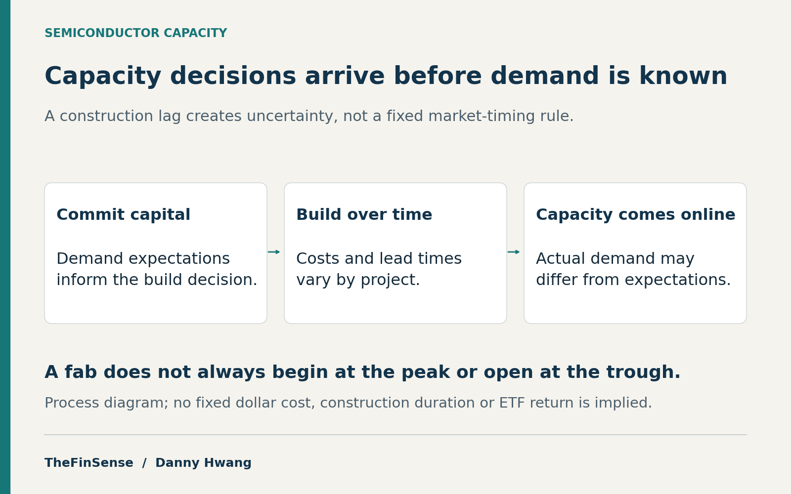
A fab gets committed to years before anyone knows whether the chips will be wanted. The forecasting problem starts there.
Why can’t analysts time the semiconductor cycle?
Capacity can arrive years after investment decisions, which makes demand and supply harder to align. That lag is one source of cyclical risk, not proof that every project arrives on the wrong side of the cycle. The same issue appears in the broader business cycle, where decision and implementation dates differ.
How do fab lead times cause the boom-bust cycle?
Fabrication capacity requires a substantial fixed investment and time to build. Cost and lead time vary by technology, location, and project. That lag can make supply and demand harder to align; it does not establish an ETF entry signal.
The NBER working paper, first issued in 2024 and revised in September 2026, documents substantial fixed fabrication investment. Separately, Intel describes its fab construction as a multiyear undertaking. These sources establish capital and construction constraints, not a fixed industry cycle or an ETF timing signal.
Eighteen years of scheduled saving produce a lower modeled endpoint after three years of delayed exposure under the assumptions below.
Formula: FV = P0*(1+r)^n + PMT*[((1+r)^n-1)/r], monthly r = annual/12
Model: delayed-start comparison of consistent monthly buying against a wait-then-invest path, valued at end of period. During the wait, the $4,000 opening balance and each saved $750 monthly contribution remain in cash and earn the selected cash rate: 0% in the base case, 4% in the cash sensitivity. At the end of the wait, the entire accumulated cash balance enters the fund at once, and later $750 monthly contributions are invested on schedule.
Assumptions: 8% nominal return scenario, cash earning 0% during the wait in the base case, and no taxes or fees modeled.
Does not apply to: single stocks, leveraged ETFs, or horizons under two years.
Regulatory catalyst: none.
The billings study and NBER working paper supply cycle context; they do not validate the model’s ETF returns or waiting-cost estimates. The scenario inputs and calculation method are stated here. See Editorial Policy.
Physical lead times help explain why semiconductor supply and demand move in cycles. Neither cited study establishes a reliable semiconductor-ETF entry signal; that evidence limit does not show that no implementable timing rule could work.
Semiconductor ETF dollar cost averaging: common questions
How long is the semiconductor cycle?
Three to four years is a historical rule of thumb, not a current peak-to-peak schedule. Tokyo Electron describes that rhythm in the computer era and notes that it changed with smartphone demand and a more diverse electronics market. Construction lead times can complicate capacity planning, but they do not fix the length or direction of the next cycle.
Did AI kill the semiconductor cycle?
AI demand does not by itself establish a future cycle length or a permanent end to downturns. Fabrication still requires capital and construction time, while the demand mix can change. Those constraints do not prove that capacity will always arrive late or overshoot. The sources here do not forecast the next AI-related turn. A purchase schedule removes discretionary entry-date decisions; it does not protect the investment’s value. Scheduled semiconductor purchases can still lose substantially if the sector falls, including when the next cycle behaves differently.
SMH vs SOXX: which is better for averaging?
Both funds concentrate exposure in the semiconductor industry. The dated official documents below identify their benchmarks and fund expenses; they do not establish which fund is best for a particular investor. Compare current holdings and weights on the same date before making a concentration claim. For broad-index context, see the Dow, Nasdaq and S&P 500 comparison.
| Ticker | Benchmark | Stated expense ratio | Document date |
|---|---|---|---|
| SMH | MVIS US Listed Semiconductor 25 Index | 0.35% net | September 30, 2026 |
| SOXX | NYSE Semiconductor Index | 0.34% | June 30, 2026 |
When is the best time to buy a semiconductor ETF?
For money allocated to a long-term semiconductor sleeve, a recurring purchase date can reduce discretionary entry decisions. First check reserves, horizon, total sector exposure, and fees. The scenario in this guide does not identify the best date or prove that scheduled buying beats waiting on every market path.
Averaging vs lump sum for cyclical sectors?
For an available lump sum, investing at once can outperform staged purchases when markets rise during the staging period; staged purchases can do better when they fall. Buying near a bottom is not required for a lump sum to win. New monthly income is a separate decision because those dollars were not available earlier. The billings study does not compare ETF funding strategies. If staging helps you follow your plan, choose the schedule after checking reserves, horizon and sector concentration.
The bottom line on semiconductor ETF dollar cost averaging
In the displayed 18-year constant-return scenario, a three-year wait produces a lower ending balance; a different market path or cash rate can change that result.
Separate the decisions before acting: recurring purchases invest new income, staged investment spreads an existing lump sum, and waiting in cash delays exposure. The calculator shows how a delay changes one assumed-return path. It does not forecast the next sector bottom or establish the historical cost of guessing it.
The same compounding that opened this gap can be watched grow month by month.
Next reads: see how the 100% US cost study runs a similar hidden tab, watch the same compound interest build the gap month by month, or read why emerging markets underperform.
YOUR TURN
When the chip sector drops next, do you have a tested, implementable entry rule, or are you simply delaying purchases?
The constant-return scenarios are reproducible from the stated formula and inputs; the cited studies provide cycle context rather than a test of the investment paths. See Editorial Policy.
Additional source context and related calculations
The reported 78% of cases concerns tests that did not reject the null of no directional information. It is not a 78% forecast-error or losing-trade rate. The models forecast world semiconductor billings, not ETF prices.
Reproducing the delayed-start comparison. Let F(P,C,i,n) = P(1 + i)^n + C[((1 + i)^n − 1)/i], using P + Cn when i is zero. Here i is the nominal annual rate divided by twelve, n is months, and contributions arrive at month end. The steady path is F(P,C,i,n).
With a wait of w months, first accumulate cash K = F(P,C,j,w), where j is the selected nominal annual cash rate divided by twelve; then invest it and continue contributions: F(K,C,i,n − w). Cap w at the horizon. The base inputs are P = $4,000, C = $750, n = 18 × 12, annual fund return 8%, w = 36, and cash return 0%. The cash sensitivity changes that last rate to 4%. Other rows change only the displayed assumption; calculate gaps from unrounded endpoints and round columns separately. There are no taxes, fees, variable returns, or timing signals. The published semiconductor-billings research provides cycle context, not empirical validation of the model’s fund returns or waiting costs.
Update history
View dated amendments
- Calculator interaction correction October 19, 2026 CORRECTION
Changing an input now clears the previous result until Calculate or Enter runs the model again. Model assumptions, formulas and published scenario values are unchanged.
- Final-reader correction October 18, 2026 CORRECTION
Removed a “Previous update: July 19, 2026” label that conflicted with the dated amendments below. Calculator, scenario inputs and results are unchanged.
- Independent-check clarification October 17, 2026 CLARIFICATION
Qualified the historical cycle rhythm, separated fab investment and construction sources, and narrowed behavioral, suitability and billings-forecast claims. Scenario inputs and results are unchanged.
- Attribution and scope clarification October 17, 2026 CLARIFICATION
Removed unsupported personal-work, compensation and holdings assertions. The delayed-start model, its inputs, numerical results and assets are unchanged.
- Article amendment October 15, 2026 CORRECTION
Renamed the five-year wait, explained cash accumulation before the first result, and linked dated issuer comparisons.
- Article amendment October 15, 2026 CORRECTION
Added an accessible canvas to the schedule chart; retained both scenario paths and their data table.
- Article amendment October 14, 2026 CORRECTION
Moved the practical investing steps and scenario before the research discussion, clarified the forecast test, and shortened repeated summaries.
- Article amendment October 14, 2026 CORRECTION
Clarified calculator input limits and added zero-return and reversal examples; distinguished the hypothetical scenario from a measured market-timing result.
- Article amendment October 14, 2026 CORRECTION
Corrected the scenario-design description and removed repeated forecasting caveats.
- Article amendment 2026-07-19 PUBLISH
Published.