
Updated:
⏱ Published · Source snapshot
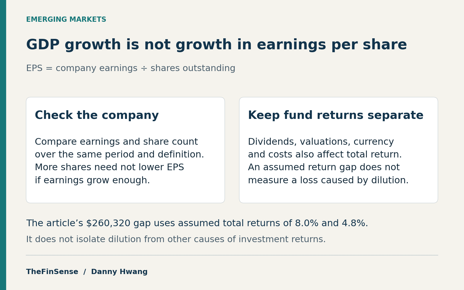
GDP growth is not earnings growth per share. Compare earnings and share count on the same basis; the $260,320 model assumes a total-return gap and does not measure a loss caused by dilution. See the EPS mechanism · Run the document checks.
Read the growth-to-shareholder explanation
Emerging markets often disappoint investors for a reason that has little to do with slow growth: economic growth does not automatically become growth in earnings per share. In many emerging markets, new share issuance has historically absorbed a large part of that growth before it reaches existing shareholders.
That is why a country’s GDP can look strong while its long-run investor returns stay weak. Per-share earnings can help test a fund’s economic-growth narrative; valuation, currency, costs, and diversification still affect the investment decision.
Browse the full guide
After fifteen years of disappointing returns, investors are again being told the emerging-market growth story is about to pay off. GDP growth alone does not establish how existing shareholders will fare. Using the dilution discussion as context, the illustrative model compares two assumed total-return paths and produces a $260,320 difference over twenty-five years. The title’s 15 markets refer to Ritter’s 1988–2011 cross-country table. J.P. Morgan’s fifteen-year EPS window and Priya’s twenty-five-year assumed-return model are separate comparisons. This is a long-run, cross-country pattern; any single market or decade can and sometimes does run the other way.
Why Don’t Booming Emerging Economies Deliver Booming Returns?
Emerging economies have often grown substantially faster than the developed world, and profits ultimately flow from economic output. Allocation models, index providers, and business-news segments repeat that growth premium as settled fact. If growth reliably reached shareholders, the fastest-growing economies would indeed be the best place to invest.
The boom is genuine. The mistake is assuming it lands in the shares you already own rather than in the new ones a growing economy keeps issuing.
Picture a company’s earnings as water and its shares as cups. More cups mean less water per cup only if the water supply does not grow enough to keep up. The same condition applies to earnings per share: added shares can reduce EPS, but earnings from the new capital can offset the increase in share count.
This analysis is written for anyone who holds or is considering an emerging-markets index fund or ETF and wants to know whether the growth story actually reaches their returns. It is less relevant to single-stock pickers or short-term traders, and it describes long-run averages rather than any one market or decade.
The economies that grew the most have often rewarded their shareholders the least.
The missing link is the difference between aggregate economic growth and earnings growth per share. For a refresher on what one share actually represents, start with what a stock really is.
How Much of Emerging-Market Growth Actually Reaches Shareholders?
The cited research reports a larger historical gap between aggregate growth and per-share earnings in emerging markets. At company level, new shares reduce an existing holder’s ownership percentage; EPS falls only if earnings fail to grow enough to offset the added shares. New listings can also change a country’s aggregate earnings base without diluting the shares of a different existing company.
Dilution is not the only force at work. Valuation changes, the price paid for expected growth, and the start date of any measurement all matter too. This guide focuses on dilution because it can be examined in per-share earnings and share-count data.
For the long-run backdrop, the Dimson-Marsh-Staunton Yearbook (2026 edition, covering 1900-2025) shows developed markets returning 8.5% a year in nominal U.S. dollar terms since 1900, versus 6.9% for emerging markets.
Faster Growth, Weaker Returns: 15 Emerging Markets
Compare all fifteen markets in the numerical table. GDP growth and real stock returns are different measures; use the country-specific periods listed below.
| Market | GDP growth | Real stock return |
|---|---|---|
| Argentina | 2.4% | 10.4% |
| Brazil | 2.0% | 13.3% |
| Chile | 4.0% | 14.1% |
| China | 9.4% | -5.5% |
| India | 5.1% | 4.1% |
| Jordan | 0.9% | 1.2% |
| Malaysia | 3.9% | 6.8% |
| Mexico | 1.2% | 15.0% |
| Philippines | 1.8% | 3.1% |
| Portugal | 1.9% | -0.9% |
| Russia | 3.6% | -6.8% |
| South Korea | 4.7% | 4.2% |
| Taiwan | 4.3% | 4.9% |
| Thailand | 4.1% | 5.4% |
| Turkey | 2.4% | 5.0% |
The historical estimates discussed here concern per-share earnings: dilution was about half a percent a year in developed markets and closer to 3.2% in emerging markets. They are not annual fees or direct deductions from an emerging-markets fund’s total return. In its November 24, 2025 report covering the preceding fifteen years, J.P. Morgan Asset Management reported, “net dilution has acted as a 400bps per year headwind to EM EPS.” One basis point is a hundredth of a percentage point, so 400 basis points is about four percentage points a year of pressure on per-share earnings. In China alone that figure reached roughly 820 basis points.
That headwind falls on earnings per share, which is not the same as a fund’s total return. Dividends, valuation swings, and currency moves all sit on top of it. But over long horizons, persistent EPS dilution is one of the clearest reasons a fast-growing market can leave its shareholders behind.
Why Does Economic Growth Skip Your Earnings Per Share?
Growth reaches an economy’s total output long before it reaches any single share. Whenever the share count grows faster than earnings, earnings per share lag behind the economy that produced them. MSCI Barra’s 1969-2009 table covered sixteen developed markets, and across those with usable earnings-per-share data it reported an average 2.3-percentage-point gap between real GDP growth and per-share earnings growth.
A company’s secondary offering adds shares immediately. If the capital raised later generates enough additional earnings, EPS need not fall. A new company’s IPO expands the listed market but does not itself dilute holders of another company. Retained earnings, debt and productivity gains are other ways to finance growth. The relevant check is what happens to matched per-share earnings, not issuance alone.
Before this work, country-allocation models often treated GDP growth as a near-direct proxy for future stock returns. Ritter, and Bernstein and Arnott, reframed growth as a ceiling that dilution and issuance erode before it reaches per-share earnings — the effect Bernstein and Arnott had already labeled the “two percent dilution.” The effect also compounds through dividends, since what a company pays per share, not in aggregate, is what an income investor actually keeps after dividend tax drag.
Apparently, consumers and workers rather than the shareholders of existing companies gain all of the benefits of economic growth.
Jay Ritter, 2012, Journal of Applied Corporate Finance
The common thread across Ritter and MSCI Barra is that a country’s economic growth and a shareholder’s per-share return are two different numbers.
Priya’s $260,320 Assumed-Return Gap
Illustrative model, not an observed loss caused by dilution: $25,000 initially plus $500 at each month-end for 25 years, comparing assumed annual returns of 8.0% and 4.8%. The $260,320 gap depends on these inputs; the model does not isolate dilution from valuation, currency or other causes.
The two paths below compare assumed total returns of 8.0% and 4.8%. The 3.2-point difference is a sensitivity input motivated by the dilution discussion, not a conversion formula from EPS dilution to fund return. Realized fund returns already include issuance effects as well as dividends, valuation, currency, and costs; subtracting the same historical EPS estimate again could double-count it.
Priya is a hypothetical 45-year-old saver with a 25-year horizon, a $25,000 start, and $500 monthly contributions. The two chosen total-return assumptions show how a persistent return difference compounds; no holdings or issuance path has been constructed for her account.
Priya is a hypothetical example, not a real individual.
| Input | Value |
|---|---|
| Age today / target age | 45 / 70 |
| Initial balance | $25,000 |
| Monthly contribution | $500 |
| Time horizon | 25 years |
| Higher assumed total return | 8.0% a year |
| Lower assumed total return | 4.8% a year (8.0% minus the 3.2% wedge) |
Formula: FV=P*(1+m)^n+C*(((1+m)^n-1)/m), with m=(1+r)^(1/12)-1. P is the starting balance, C the month-end contribution, r the annual effective return and n the number of months. If m=0, use P+C*n.
Model: higher versus lower assumed-total-return compounding, calculated monthly, end of period.
Assumptions: 8.0% and 4.8% are illustrative annual total returns. Their 3.2-percentage-point separation is a sensitivity choice. The separately cited historical EPS dilution estimate does not determine a fund-return deduction.
Does not apply to: single-market or single-decade outcomes.
| Year | Higher assumed return | Lower assumed return | Gap |
|---|---|---|---|
| Year 5 | $73,206 | $65,346 | $7,859 |
| Year 10 | $144,035 | $116,351 | $27,684 |
| Year 15 | $248,107 | $180,829 | $67,278 |
| Year 20 | $401,023 | $262,342 | $138,682 |
| Year 25 | $625,707 | $365,387 | $260,320 |
The two paths are illustrative, not forecasts. Their purpose is to show how a persistent assumed total-return difference can compound over a long holding period, which you can watch by visualizing compound interest side by side.
| Year | Higher assumed return | Lower assumed return |
|---|---|---|
| Year 5 | $73,206 | $65,346 |
| Year 10 | $144,035 | $116,351 |
| Year 15 | $248,107 | $180,829 |
| Year 20 | $401,023 | $262,342 |
| Year 25 | $625,707 | $365,387 |
China is the sharpest version of this story, and it comes with a caveat worth stating up front. Using Ritter’s 2012 MSCI-based data, China’s real per-capita GDP grew roughly fivefold while its shareholders lost money in real terms, near -5.5% a year. Later work by Hsu and colleagues, using mainland A-share returns over 1993-2019, puts China’s real return modestly positive. Both the return series and the endpoint differ from Ritter’s 1993-2011 comparison, so the difference cannot be attributed to the series alone.
Start from the base case of $25,000, $500 monthly and 25 years. Each row changes only the input named in its “What changed” cell; all other inputs stay at the base case. The higher and lower columns are assumed total-return paths, not the payoff from a tested screening strategy. The 2.3-point row is a separate illustrative return input, not a developed-market dilution floor. The 4.0- and 8.2-point inputs echo the cited EPS discussion but are not estimates of fund-return deductions. The 8.2-point assumption makes the lower modeled return slightly negative.
Sensitivity table: 11 scenarios
| Scenario | What changed | Higher assumed return | Lower assumed return | Gap |
|---|---|---|---|---|
| Base case | Setup: P=$25K, PMT=$500/mo, t=25y, r=8.0%, wedge=3.2pp | $625,707 | $365,387 | $260,320 |
| Shallower wedge | assumed return gap 2.3pp; not an EM dilution floor | $625,707 | $423,730 | $201,977 |
| Deeper wedge | assumed return gap 4.0pp; separate from JPM EPS estimate | $625,707 | $321,070 | $304,637 |
| China wedge | assumed return gap 8.2pp; not measured China fund drag | $625,707 | $170,100 | $455,608 |
| Lower base | r 7.0% (lower base return) | $527,207 | $310,973 | $216,234 |
| Higher base | r 9.0% (higher base return) | $744,420 | $430,833 | $313,586 |
| Shorter horizon | t 20y | $401,023 | $262,342 | $138,682 |
| Longer horizon | t 30y | $955,842 | $495,654 | $460,188 |
| Lighter saver | PMT $250/mo | $398,460 | $223,053 | $175,407 |
| Heavier saver | PMT $750/mo | $852,955 | $507,721 | $345,234 |
| Larger lump | P $50K | $796,919 | $446,105 | $350,814 |
The 8.2-point sensitivity sets the lower assumed total return at −0.2% and gives a $455,608 gap. It is the most severe assumption shown, not an estimate of what Chinese issuance costs a fund investor.
The $260,320 is the difference between two assumed-return projections. It is not missing capital observed in an account, and the model does not establish that dilution caused an investor to lose that amount.
How Should You Actually Invest in Emerging Markets?
The dilution evidence is a reason to inspect how growth reaches existing shareholders. It does not establish that a particular selection screen improves fund returns, nor does it settle whether an emerging-market allocation fits your portfolio.
Start dates cut both ways. Measured in nominal U.S. dollar terms since 1960, emerging markets led at 10.9% a year against developed markets’ 9.6%, so the winner flips depending on where you start the clock.
Step 1: Measure Dilution Directly
Measure dilution at the level that actually matters. Do not use the ETF’s own shares outstanding, which mostly track fund flows and the creation-redemption process, not the dilution of the companies it holds. Look instead at the index’s net equity issuance, or the weighted change in shares outstanding across the fund’s underlying companies. Ritter’s 2012 study compared per-capita GDP growth against real equity returns and found them negatively correlated. A country’s headline growth rate does not establish the return existing shareholders receive.
How to find the inputs: start on your fund provider’s product page and record the exact benchmark name, holdings date and any published EPS or net-issuance history. Open that index provider’s factsheet or research archive and look for a comparable per-share earnings series and a stated net-issuance measure; if these are not public, ask the provider rather than inferring them from the ETF’s own unit count. For a holding-level check, use the disclosed constituent list to open company investor-relations annual reports, or SEC EDGAR filings where available, and locate EPS, the share-count note and the statement of changes in equity.
Compare the same fiscal years, share class and accounting basis. Separate basic from diluted EPS and weighted-average EPS share counts from shares outstanding on a single date; account for splits and changes in the holdings before comparing periods. Do not add constituent EPS figures or call a changing-weight fund a fixed-company issuance series. If comparable index history or sufficient company coverage is unavailable, record the dilution diagnostic as unknown and keep the allocation decision anchored to valuation, costs, currency and diversification. This document check does not establish a superior fund-selection screen.
Step 2: Compare EPS With the Growth Claim
Compare per-share earnings with the growth story being offered. Hsu and colleagues study the relationship between EPS growth and emerging-market returns; the result does not by itself establish an implementable fund-selection rule. Check the benchmark, period, valuation, and share-count basis before interpreting an EPS trend.
Step 3: Interpret Issuance Alongside Earnings
Use the matched share-count and EPS records gathered in Step 1 to test the forecast. Added shares are a warning to investigate, not proof of lower returns: earnings from the new capital can offset the increase.
Step 4: Review Total Portfolio Exposure
Review the position alongside the portfolio’s country, sector and currency exposures, valuation and fees. The model does not determine an allocation size or show how much a screening rule would recover.
EPS growth, net share issuance, and dividends per share help evaluate a growth claim, but no one of them establishes the best fund. Also compare valuation, currency, governance, sector exposure, fees, and diversification. Dividend yield traps show why a high quoted payout can distract from a weaker business.
Checking issuance and earnings per share can clarify how growth reaches existing shareholders. This article has not tested whether screening for those traits improves future fund returns or closes the $260,320 modeled gap. Ask whether EPS and share count support the growth story, then also check valuation, currency, costs, and portfolio concentration.
Emerging Markets: Frequently Asked Questions
Does GDP growth lead to higher stock returns?
GDP growth does not reliably lead to higher stock returns, and across countries the relationship has been weak or negative. Jay Ritter reported a negative correlation between real per-capita GDP growth and real stock returns: about -0.39 for 19 developed markets over 1900 to 2011, and about -0.41 for 15 emerging markets over 1988 to 2011. China is the clearest case: using Ritter’s MSCI-based series, its real per-capita GDP grew close to 10% a year from 1993 to 2011 while its real stock return was about -5.5%, though later A-share-based work makes that figure less extreme. Output can benefit workers, consumers and newly listed firms as well as existing shareholders. For a company already held, compare earnings growth with share-count growth.
How does dilution lower emerging-market returns?
Share issuance can dilute existing holders’ earnings per share when the new capital does not generate enough additional earnings. The cited Schroders estimate is roughly 3.2% a year for historical EPS dilution, compared with 0.5% in developed markets; these are not annual deductions from a fund’s total return. The separate J.P. Morgan figures concern EPS headwinds over its stated fifteen-year sample, not a measured investor-account loss.
Should I avoid emerging markets entirely?
The dilution evidence alone does not settle whether to hold emerging markets; diversification, valuation, currency and portfolio risk still matter. A useful diagnostic is to inspect what dilution leaves behind; this is not a tested promise of better future fund returns. Hsu and colleagues’ 2022 study found a stronger same-period cross-country association between EPS growth and stock returns than between GDP growth and returns. This was a historical comparison, not an out-of-sample forecasting test. An EPS trend helps assess the growth claim; this article does not establish that selecting funds by that trend improves future returns.
The Bottom Line on Why Emerging Markets Underperform
Across the cited country samples, faster economic growth did not reliably translate into higher returns for existing shareholders. Ritter compared economic growth with shareholder returns across 34 markets and found a negative cross-country correlation in both his developed-market and emerging-market samples. Dilution is a leading reason. New shares reduce existing ownership percentages, but the effect on EPS depends on the additional earnings the capital produces. A growing listed market also includes new firms that were not previously available to existing investors. That is why shareholder-level checks are useful alongside a forecast, while their ability to improve future fund selection remains untested here. Judge an emerging-market fund by the earnings-per-share growth and the net-issuance trend of its underlying holdings, not by the GDP number its country is projected to post.
Use matched company or index documents to test the per-share growth story. The modeled $260,320 difference illustrates compounding under two assumed total returns and does not measure capital lost to issuance.
Before you trust an emerging-markets fund’s growth story, check the index’s EPS growth and the net issuance trend of its underlying companies, not the ETF’s own unit count.
Next: compare a 100% US portfolio with a global allocation under stated return assumptions.
Reproducing the assumed-return model. Use FV(P, C, r, n) = P(1 + m)^n + C[((1 + m)^n − 1)/m], where m = (1 + r)^(1/12) − 1, n is the number of months, P is the starting balance, and C is the end-of-month contribution. When m is zero, use P + Cn. The base case is P = $25,000, C = $500, n = 25 × 12, with annual rates 8.0% and 4.8%.
The lower rate is the higher rate minus the selected percentage-point wedge. Each sensitivity row changes only its stated input and keeps the other case inputs fixed; the slightly negative China-wedge rate uses the same formula. Compute each gap before rounding the columns independently to whole dollars. These are constant assumed total-return paths, not GDP forecasts or a tested screening strategy. They exclude taxes, fees, changing returns, and sequence risk; a historical dilution average does not establish a future fund-return shortfall.
Financial disclosure: Nothing above is a recommendation to buy or sell any security.
This article is educational and not personalized financial, tax, or investment advice. The dollar figures are illustrative projections built on an assumed return, not forecasts or guarantees. Emerging-market investing carries real risk of loss. Consult a licensed advisor before acting, and remember that past performance does not predict future results.
Update history
View dated amendments
- Final-reader correction October 18, 2026 CORRECTION
Stated Ritter’s two correlation samples separately (about -0.39 for developed markets, 1900–2011; about -0.41 for emerging markets, 1988–2011) instead of describing the relationship as slight, and pointed the byline SSRN link to the cited paper. Scenario inputs and results are unchanged.
- Independent-check clarification October 17, 2026 CLARIFICATION
Specified currency and country windows, distinguished per-capita growth and research periods, replaced a forecasting claim with historical association, and removed an unmatched benchmark comparison. Numerical results are unchanged.
- Rounding correction October 17, 2026 CORRECTION
Corrected the five-year assumed-return gap to $7,859 by subtracting unrounded balances before display rounding. The displayed endpoint balances, model inputs and other results are unchanged.
- Attribution and scope clarification October 17, 2026 CLARIFICATION
Made the share-issuance analogy conditional on earnings growth and removed unsupported personal-work, compensation and holdings assertions. Historical observations, scenario inputs, calculations and assets are unchanged.
- Article amendment October 15, 2026 CORRECTION
Separated market count from measurement periods, corrected sensitivity descriptions, and kept issuance conclusions conditional.
- Article amendment October 15, 2026 CORRECTION
Added accessible canvases to both existing charts; historical data, assumed-return paths and numerical tables are unchanged.
- Article amendment October 14, 2026 CORRECTION
Changed the currency companion anchor from a claimed realized investor cost to its actual matched-index and scenario scope.
- Article amendment October 14, 2026 CORRECTION
Removed the remaining FAQ implication that an EPS estimate is a measured fund-return charge.
- Article amendment October 14, 2026 CORRECTION
Separated assumed fund-return scenarios from historical EPS findings and clarified the table and figure descriptions.
- Article amendment October 14, 2026 CORRECTION
Recast EPS checks as diagnostics rather than a tested fund-selection rule; distinguished assumed return gaps from EPS measures.
- Article amendment July 16, 2026 CORRECTION
Corrected four one-dollar table discrepancies, made the historical comparison chart accessible, removed unsupported lifestyle and country claims, and updated the J.P. Morgan source.
- Article amendment July 13, 2026 CORRECTION
corrected Dimson-Marsh-Staunton citation to the 2026 Yearbook (1900-2025); clarified that the 3.2% dilution wedge is an EPS-level, illustrative figure rather than a guaranteed total-return cost; moved the China return caveat to first mention; streamlined the layout.
- Article amendment July 12, 2026 PUBLISH
initial publication.